Seurat不仅可以校正实验的批次效应，还能跨平台整合数据，例如将10x单细胞数据、BD单细胞数据和SMART单细胞数据整合在一起；也能整合单细胞多组学数据，例如将单细胞ATAC、空间转录组与单细胞转录组数据整合在一起。（甚至可以跨物种整合）
scRNA-seq%E6%95%B0%E6%8D%AE%E6%95%B4%E5%90%88Introduction%20db516adcc0714bf29501a8f3f63c0f58/Untitled%208.png
参考链接: https://satijalab.org/seurat/articles/integration_introduction.html#introduction-to-scrna-seq-integration-1

整合数据的目的

创建一个整合后的数据进行下游分析
识别两个数据集中都存在的细胞类型
获得在对照组和受刺激组均存在的细胞类型标记（cell type markers）
比较数据集，找出对刺激有反应的特殊细胞类型（cell-type）

新建Seurat对象

使用[SeuratData](https://github.com/satijalab/seurat-data)包下载并载入示例数据

InstallData的过程其实是在下载数据，网络质量不好的情况下会比较慢。下载好后自动安装

> InstallData("ifnb")
Installing package into ‘C:/Users/xcxr/Documents/R/win-library/4.0’
(as ‘lib’ is unspecified)
试开URL’http://seurat.nygenome.org/src/contrib/ifnb.SeuratData_3.1.0.tar.gz'
Content type 'application/octet-stream' length 413266233 bytes (394.1 MB)
downloaded 394.1 MB

* installing *source* package 'ifnb.SeuratData' ...
** using staged installation
** R
** data
*** moving datasets to lazyload DB
** inst
** byte-compile and prepare package for lazy loading
** help
*** installing help indices
  converting help for package 'ifnb.SeuratData'
    finding HTML links ... 好了
    ifnb                                    html  
** building package indices
** testing if installed package can be loaded from temporary location
*** arch - i386
*** arch - x64
** testing if installed package can be loaded from final location
*** arch - i386
*** arch - x64
** testing if installed package keeps a record of temporary installation path
* DONE (ifnb.SeuratData)

The downloaded source packages are in
    ‘C:\Users\xcxr\AppData\Local\Temp\RtmpWkyo7s\downloaded_packages’
There were 48 warnings (use warnings() to see them)

warnings 信息出现：In if (is.na(desc)) { ... : 条件的长度大于一，因此只能用其第一元素 其含义不明

library(Seurat)
# devtools::install_github('satijalab/seurat-data')
library(SeuratData)
library(patchwork)
library(tibble)

# install dataset
InstallData("ifnb")
# load dataset
LoadData("ifnb")

# ifnb 是一个seurat对象
> ifnb
An object of class Seurat 
14053 features across 13999 samples within 1 assay 
Active assay: RNA (14053 features, 0 variable features)

# split the dataset into a list of two seurat objects (stim and CTRL)
ifnb.list <- SplitObject(ifnb, split.by = "stim")

# ifnb.list中含有两个元素，分别是CTRL和STIM
> ifnb.list
$CTRL
An object of class Seurat 
14053 features across 6548 samples within 1 assay 
Active assay: RNA (14053 features, 0 variable features)

$STIM
An object of class Seurat 
14053 features across 7451 samples within 1 assay 
Active assay: RNA (14053 features, 0 variable features)

使用lapply()函数对列表内的元素分别进行归一化和高变基因识别：

# normalize and identify variable features for each dataset independently
ifnb.list <- lapply(X = ifnb.list, FUN = function(x) {
    x <- NormalizeData(x)
    x <- FindVariableFeatures(x, selection.method = "vst", nfeatures = 2000)
})

SelectIntegrationFeatures()函数返回在多组数据集中重复变化的基因，用于下一步寻找组间的Anchors，object.list参数指定需要整合的数据组列表，数据类型必须是seurat object；可以用nFeatures参数指定返回的基因数量。（对于未运行过的FindVariableFeatures()的对象，会自动运行，寻找高变基因）

# select features that are repeatedly variable across datasets for integration
features <- SelectIntegrationFeatures(object.list = ifnb.list)

多组数据先各自进行QC和归一化后再进行整合。

开始整合 Perform integration

FindIntegrationAnchors()函数导出多组数据之间的Anchors（Anchors是Seurat进行多组数据整合的核心概念，翻译成汉语叫做锚也就是基于CCA的一种数据比对（alignment）的方法，替代了之前版本的RunCCA()函数）

参数 scale: Whether or not to scale the features provided. Only set to FALSE if you have previously scaled the features you want to use for each object in the object.list 只有在合并数据之前就已经将各组数据分别标准化了才设为FALSE，否则保持默认。

immune.anchors <- FindIntegrationAnchors(object.list = ifnb.list, anchor.features = features)
# this command creates an 'integrated' data assay
immune.combined <- IntegrateData(anchorset = immune.anchors)

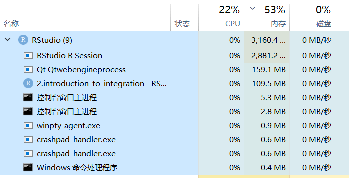
ps：运行完这一步，发现R占用的内存已经达到3G了！看来用不起服务器的情况下，以后做多样本的处理还得加个内存条啊！不过整合后的数据进行下游分析应该只要用到immune.combined这个数据，如果可以直接把其导出直接分析。

整合后的数据分析 Perform an integrated analysis

整合以后我们就可以对所有的细胞一起分析，分析思路和方法与之前的 Seurat基本分析流程一样。

我们可以看到immune.combined这个对象的assays现在有两个，其中RNA是原始的数据，integrated是我们上一步使用anchors进行整合后的数据，在下游分析中需要使用integrated的是数据，所以使用DefaultAssay() ← ？指定默认的assay。接下来就是按照标准流程进行探索。

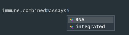
scRNA-seq%E6%95%B0%E6%8D%AE%E6%95%B4%E5%90%88Introduction%20db516adcc0714bf29501a8f3f63c0f58/Untitled%201.png

# specify that we will perform downstream analysis on the corrected data note that the original
# unmodified data still resides in the 'RNA' assay
DefaultAssay(immune.combined) <- "integrated"

# Run the standard workflow for visualization and clustering
immune.combined <- ScaleData(immune.combined, verbose = FALSE)
immune.combined <- RunPCA(immune.combined, npcs = 30, verbose = FALSE)
immune.combined <- RunUMAP(immune.combined, reduction = "pca", dims = 1:30)
immune.combined <- FindNeighbors(immune.combined, reduction = "pca", dims = 1:30)
immune.combined <- FindClusters(immune.combined, resolution = 0.5)

可视化：

# Visualization
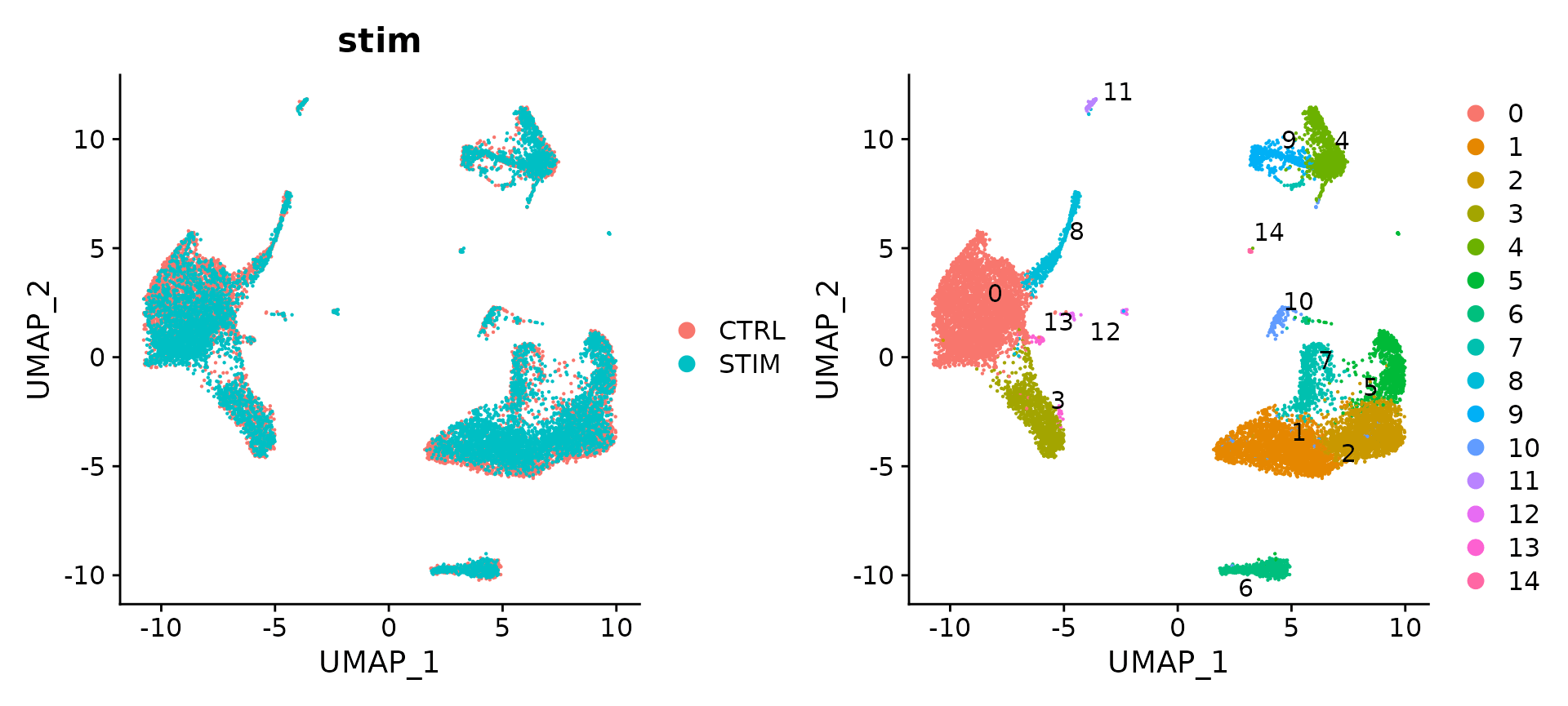
p1 <- DimPlot(immune.combined, reduction = "umap", group.by = "stim")
p2 <- DimPlot(immune.combined, reduction = "umap", label = TRUE, repel = TRUE)
p1 + p2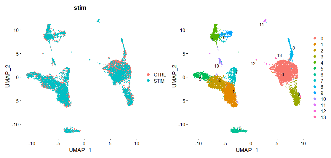

scRNA-seq%E6%95%B0%E6%8D%AE%E6%95%B4%E5%90%88Introduction%20db516adcc0714bf29501a8f3f63c0f58/Untitled%202.png

实际运行出来的图

scRNA-seq%E6%95%B0%E6%8D%AE%E6%95%B4%E5%90%88Introduction%20db516adcc0714bf29501a8f3f63c0f58/Untitled%203.png

官方教程配图

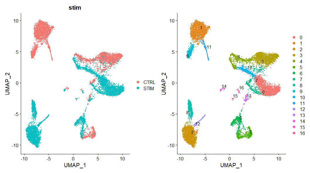
这里我们可以尝试一下如果不使用seurat进行整合，得出的细胞分群是什么样的：

# try without integration
ifnb <- ifnb
ifnb <- NormalizeData(object = ifnb, normalization.method = "LogNormalize", scale.factor = 1e4)
ifnb <- FindVariableFeatures(ifnb, selection.method = "vst", nfeatures = 2000)
all.genes <- rownames(ifnb)
ifnb <- ScaleData(ifnb, features = all.genes)
ifnb <- RunPCA(ifnb, npcs = 30)
ifnb <- RunUMAP(ifnb, reduction = "pca", dims = 1:30)
ifnb <- FindNeighbors(ifnb, reduction = "pca", dims = 1:30)
ifnb <- FindClusters(ifnb, resolution = 0.5)
p1 <- DimPlot(ifnb, reduction = "umap", group.by = "stim")
p2 <- DimPlot(ifnb, reduction = "umap", label = TRUE, repel = TRUE)
p1 + p2

scRNA-seq%E6%95%B0%E6%8D%AE%E6%95%B4%E5%90%88Introduction%20db516adcc0714bf29501a8f3f63c0f58/Untitled%204.png

without integration

可以看出两个样本中的细胞不能map到一起，与整合后的效果差异很明显。

如果需要把对照组（CTRL）和处理组（STIM）分开单独进行可视化，可以使用split.by参数指定分组。

DimPlot(immune.combined, reduction = "umap", split.by = "stim")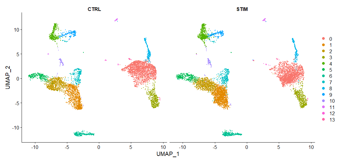

scRNA-seq%E6%95%B0%E6%8D%AE%E6%95%B4%E5%90%88Introduction%20db516adcc0714bf29501a8f3f63c0f58/Untitled%205.png

鉴定组间保守的细胞标记物 Identify conserved cell type markers

对整合后的数据组分析结束后，再回到原始数据（DefaultAssay(x)<- "RNA"）来寻找保守的细胞标记物。

# For performing differential expression after integration, we switch back to the original data
DefaultAssay(immune.combined) <- "RNA"
nk.markers <- FindConservedMarkers(immune.combined, ident.1 = 6, grouping.var = "stim", verbose = FALSE)
head(nk.markers)

FindConservedMarkers() 分析保守标记物需要调用multtest和metap包，如果没有提前安装会报错。教程中操作的时候是已经知道了cluster6是nk细胞，实际探索过程中，一般不会提前知道细胞种类，所以通常使用cluster0.markers <- FindConservedMarkers()，逐一计算保守标记物。

> nk.markers <- FindConservedMarkers(immune.combined, ident.1 = 6, grouping.var = "stim", verbose = FALSE)
错误: Please install the metap package to use FindConservedMarkers.
This can be accomplished with the following commands: 
----------------------------------------
install.packages('BiocManager')
BiocManager::install('multtest')
install.packages('metap')
----------------------------------------

上面两个包安装完了之后再运行，程序提示FindMarkers默认使用Wilcoxon 秩和检验方法，建议安装limma包，检验效率会更高（🙂像极了一个推销员）。不过此时程序已经在运行，几分钟后环境变量中会出现nk.markers

> nk.markers <- FindConservedMarkers(immune.combined, ident.1 = 6, grouping.var = "stim", verbose = FALSE)
For a more efficient implementation of the Wilcoxon Rank Sum Test,
(default method for FindMarkers) please install the limma package
--------------------------------------------
install.packages('BiocManager')
BiocManager::install('limma')
--------------------------------------------
After installation of limma, Seurat will automatically use the more 
efficient implementation (no further action necessary).
This message will be shown once per session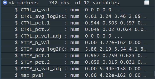

scRNA-seq%E6%95%B0%E6%8D%AE%E6%95%B4%E5%90%88Introduction%20db516adcc0714bf29501a8f3f63c0f58/Untitled%206.png

> head(nk.markers)
       CTRL_p_val CTRL_avg_log2FC CTRL_pct.1 CTRL_pct.2 CTRL_p_val_adj    STIM_p_val STIM_avg_log2FC
GNLY            0        6.006173      0.944      0.045              0  0.000000e+00        5.856524
FGFBP2          0        3.243588      0.505      0.020              0 4.224915e-162        2.187640
CLIC3           0        3.461957      0.597      0.024              0  0.000000e+00        3.540011
PRF1            0        2.650548      0.422      0.017              0  0.000000e+00        4.100285
CTSW            0        2.987507      0.531      0.029              0  0.000000e+00        3.136218
KLRD1           0        2.777231      0.495      0.019              0  0.000000e+00        2.865059
       STIM_pct.1 STIM_pct.2 STIM_p_val_adj      max_pval minimump_p_val
GNLY        0.957      0.059   0.000000e+00  0.000000e+00              0
FGFBP2      0.259      0.015  5.937273e-158 4.224915e-162              0
CLIC3       0.623      0.031   0.000000e+00  0.000000e+00              0
PRF1        0.864      0.057   0.000000e+00  0.000000e+00              0
CTSW        0.596      0.035   0.000000e+00  0.000000e+00              0
KLRD1       0.552      0.027   0.000000e+00  0.000000e+00              0

为什么p值很多都是0？
说明显著性特别高，p值极小
marker基因在这群细胞中只有50%左右的细胞表达，也能够称为marker吗？如何选择合适的细胞marker？为什么示例数据中min.pct参数都选择0.25？
min.pct初始可以保持默认的0.1，后面酌情提高，但是过高的话会导致某些表达量低的marker被掩盖，＜0.25是比较合适的。
建议寻找pct.1和pct.2之间表达差异较大的标记基因，以及较大的倍数变化。例如，如果pct.1 = 0.90，pct.2 = 0.80，可能就不是那么需要注意的标记基因。然而，如果pct.2=0.1的话，差异更大，更有说服力。另外，如果大多数表达该标记的细胞在感兴趣的聚类中是比较有意义的。如果pct.1很低，比如0.3，可能就没有那么值得注意了。

FeaturePlot()函数用于绘制基因在降维图上的表达情况（彩点表示表达该基因的细胞），features 参数指定要绘制的特征向量，内容可以是①测序方法的特征，如基因；②元数据中的列名，如线粒体百分比；③降维对象的列名，如PC_1。min.cutoff参数？

FeaturePlot(immune.combined, features = c("CD3D", "SELL", "CREM", "CD8A", "GNLY", "CD79A", "FCGR3A", 
    "CCL2", "PPBP"), min.cutoff = "q9")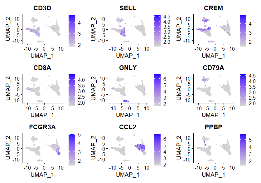

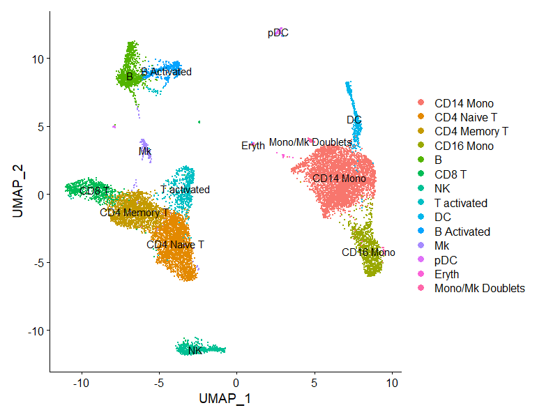
scRNA-seq%E6%95%B0%E6%8D%AE%E6%95%B4%E5%90%88Introduction%20db516adcc0714bf29501a8f3f63c0f58/Untitled%207.png

immune.combined <- RenameIdents(immune.combined, `0` = "CD14 Mono", `1` = "CD4 Naive T", `2` = "CD4 Memory T", 
    `3` = "CD16 Mono", `4` = "B", `5` = "CD8 T", `6` = "NK", `7` = "T activated", `8` = "DC", `9` = "B Activated", 
    `10` = "Mk", `11` = "pDC", `12` = "Eryth", `13` = "Mono/Mk Doublets", `14` = "HSPC")
DimPlot(immune.combined, label = TRUE)

scRNA-seq%E6%95%B0%E6%8D%AE%E6%95%B4%E5%90%88Introduction%20db516adcc0714bf29501a8f3f63c0f58/Untitled%208.png

文章版权归作者所有，转载请注明来源。

THE END

单细胞
# R # scRNA-seq # Seurat

评论共4条

欢迎您留下宝贵的见解！

提交

查看全部

- Vamond作者0
  这个笔记已经是两年多以前的了，有些信息可能存在过时的可能，建议结合seurat官方的Vignettes一起看。
  2年前@da回复
- Vamond作者0
  1. ident.1 一次只评估一个亚群，不要用(0:6)。 2. 原文中用的是 nk.markers <- FindConservedMarkers(immune.combined, ident.1 = 6, grouping.var = "stim", verbose = FALSE)，也就是用亚群6与其他所有亚群做差异分析，得到6群的标记物。 3. 原文中因为已知6群是NK细胞，所以命名变量的时候使用的是nk.markers，如果想看其他群细胞最好重新命名，以免混淆。实际使用这个函数的时候一般会写个循环，一次性把所有的标记物计算出来。 4. 如果你选择ident.1=(0:6) 是想要合并这个七群细胞计算他们统一的标记物，请先做合并处理。
  2年前@da回复

scRNA-seq数据整合Introduction

整合数据的目的

新建Seurat对象

开始整合 Perform integration

整合后的数据分析 Perform an integrated analysis

鉴定组间保守的细胞标记物 Identify conserved cell type markers